[ For my technical friends, this may be seen as straightforward. For others, I hope you find this a useful example of the type of analysis that is behind the design and maintenance of many modern products and services]

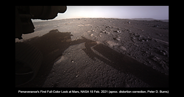
First sounds from Mars: Recently NASA posted the first audio recordings from the Perseverance rover. In order for us to hear the ambient Martian sound, two versions of the audio file were posted;

• the original, containing ‘rover self-noise’
• a version with the rover self-noise filtered out

Commenting on these sounds, Matt Heck suggested that, in general, attaching a microphone to engines is a useful part of monitoring and diagnosis of problems, wear, etc. He also suggested identifying conditions by frequency analysis to monitor resonant vibrations (frequencies). While this is often done in design, it is rare in normal product usage.

Our friend Fourier: A common analysis tool for signals of many kinds is Fourier analysis. Simply put, expressing signal/image content in terms of frequency components is another way to describe them. Whenever you hear someone say, ‘I don’t have the bandwidth to take on that task’, they are (usually inadvertently) giving a nod to the French mathematician, Joseph Fourier* … but I digress.

The Sound of the Machine: Since NASA posted the original (with-Rover) and filtered (without-Rover*) versions, let’s take a look at these signals. The audio signals are plotted here. The clip runs 18 sec., sampled at 48 kHz.

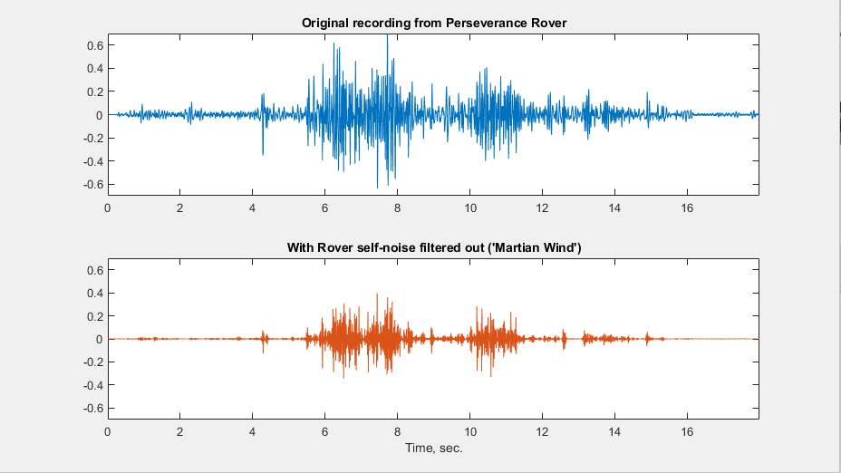
We note that the components of the apparent Martian atmospheric sounds (at 6-8 and 10-11 sec.) are evident in both records. Filtering signals such as these, under field conditions, is naturally challenging and it is not surprising that the atmospheric and machine sounds would not be completely isolated.

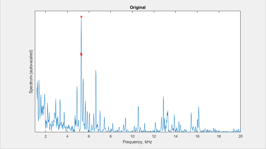
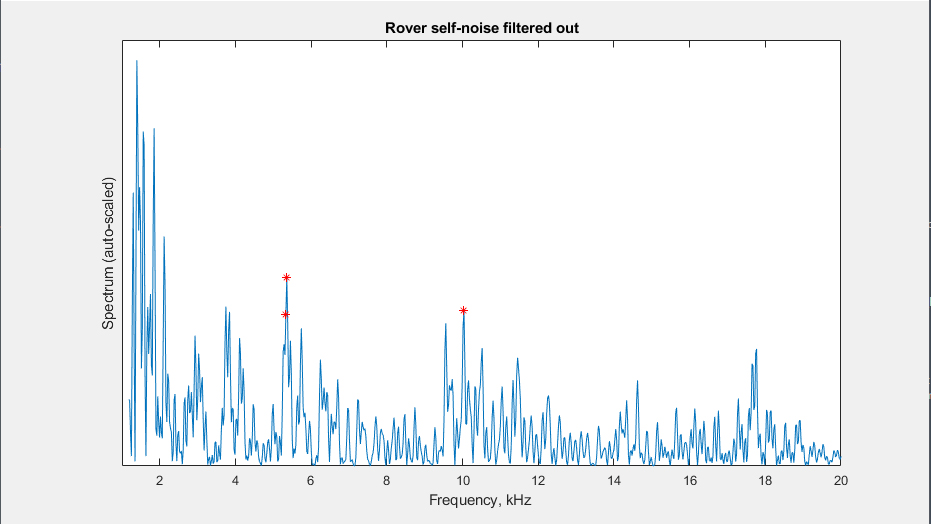
Fourier (Frequency-domain) Analysis: Consistent with Matt Heck’s suggestion, I computed the Signal (frequency) spectrum for the estimated Rover sound. [Since the statistics are not stationary, a spectrum based on a moving window is commonly used. In this case, a length 2000 FFT was used with a one-third overlap]

Shown below is the power spectral density (magnitude-squared) for a single half-second record, for both original and filtered versions. I have found the highest three components, as candidates for identification. For simplicity, the y-axes are auto-scaled, so the actual amplitude values for the two plots are different.

Variation: The results of the above analysis are subject to normal signal variation and background noise. So, to get a feel for the consistency (or underlying signature) of, e.g., the characteristic sounds that Matt Heck was referring to, I offer this short video.

The video includes the spectral analysis, here. (You might want to try it with headphones or earbuds)

Here is a version without me talking, Link

Consistent high spikes in the spectra indicate the presence of periodic components (tones) that can be tied to particular mechanisms (e.g., vibrations, motor rotation, etc.). For the original recording, we observe these at 5-7 kHz and near 13 kHz.

Other observations: 0.22 sec. of silence at the beginning, and a small delay (phase-shift) introduced by the filtering.

– Peter Burns

——

* Full name: Jean-Baptiste-Joseph Fourier