At IS&T’s Archiving 2026 Conference in Boston, Don Williams and I will be presenting our workshop. Here are the areas that we plan on covering.
This is a theory-to-practice workshop with emphasis on practice. The lecturers have more than fifty years of combined digital and analog imaging experience with ISO standards, industry, and large international libraries. We will be using Golden Thread NXT software and Photoshop for demonstration purposes
Primer on performance metrics
– Accuracy vs. consistency. What’s more important ?
– What exactly is being evaluated and why do things go wrong
– Can we create our guidelines ?
– How to recognize camera hardware from image processing influences.
– When to overlook certain imaging performance problems.
You can observe a lot just by watching.
-Learn how to visually detect JPEG, de-mosaicing, oversharpening, and noise cleaning artifacts that are not addressed in today’s current guidelines.
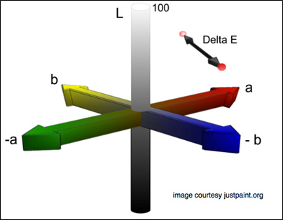
Color profiling
– Simple ways to think of color profiles. It’s not complicated.
– The underlying variables in creating color profiles
– The difference between a color profile and a color space and how to connect them.
-What are the benefits, or not, of separate profiling and verification targets?
– How can multiple target scans be combined into a single super profile.
– Understand how lighting illuminants, especially LEDs, can dramatically influence the true colorimetric (Lab, and XYZ) values that color profiles are built upon.
– How color profiling can improve goodness ratings or introduce artifacts
– How does today’s LED lighting influence true colorimetric (Lab or XYZ) values
Spatial Frequency Response
– How to interpret them and how they can vary.
– Methods for using resolution wedges for identifying de-mosaicing artifacts

